Pioneer 10 anomaly calling into question Einstein’s second postulate

Based on the anomalous acceleration acting on Pioneer 10 with a magnitude of 8.7×10^-10 m/s² directed towards the Sun, we can demonstrate that there is serious indication that the anomaly is due to the use of a wrong Doppler shift formula by the NASA Jet Propulsion Laboratory (JPL).

Indeed if we compare the result given by the formula used by JPL based on the Einstein’s second postulate, and the result given by the classic Galilean velocity addition formula, we found exactly the value of the anomalous acceleration acting on Pioneer 10 toward the Sun.

I – How did JPL discovered the ∼8 ×10⁻¹⁰ m/s² anomalous acceleration?

In the Pioneer 10 mission a ground station was sending a radio signal with frequency f_t  to the probe, then the signal was sending back synchronously to the ground station which received it at the frequency f_r.

With the Doppler shift of the radio signal, JPL was able to calculate very precisely the speed of the probe, and with the evolution of the speed they had the acceleration which was more precisely a deceleration as the probe was attracted by the whole Solar system.

With that attraction, according to the universal law of gravitation and the well-known positions of the Sun, planets and all masses in the solar system, they calculated very precisely how far was the probe from us.

The problem is that one second later the velocity of the probe should have decelerated of exactly that gravity attraction they just calculated, but no, it has decelerate a small amount more, very small, ∼ 8.7 ×10⁻¹⁰ m/s², but still, it was not normal.

II – Relativistic Doppler shift formula used by JPL

The formula used by JPL was the well-known relativistic Doppler shift formula which is:

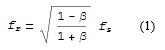
With f_s the sent frequency, fr the received frequency, β=v ⁄ c and v the velocity between the emitter and the receptor.

As there is two way for the signal, up to the probe, and down sent back synchronously to the ground station, the total round trip formula is:

And with that JPL was able to deduce the velocity v of the probe:

III – Classic Galilean Doppler shift formula:

For the way up of the signal to the probe, with v the velocity of the probe going away from the Earth, (let’s temporary consider that the Earth is stationary with the Sun as we will see that it’s equilibrates itself on the long-term, evolving from -30 km.s^-1 to   +30 km.s^-1) the formula is:

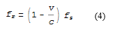
For the return trip of the signal, in the classical Galilean referential, the probe is stationary and is sending the signal with the speed of c in its reference frame toward the Earth which is moving away from it with the velocity v, so the return formula is the same, and total round trip formula is:

Let’s consider that the Galilean formulas are the good one. In that case JPL would still calculate the probe velocity with (3) but the received frequency fr would depend of a different « real velocity » than the one found by JPL and we can express the velocity calculated by JPL, V_jpl  with the « real velocity » v of the probe (two different velocity, one « real » and, from it, another one « calculated by JPL ») :

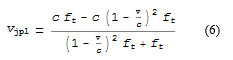
Which can be simplified not depending of the sent frequency f_s to:

IV – Solar system attraction calculation:

The solar system is attracting the probe with the respect of the universal gravitation law with all its masses M and the distance d to the probe:

As (8) is the real acceleration, each second the real velocity is changing to v – a and the velocity calculated by JPL V_jpl  expressed with the real velocity is changing to:

At the beginning JPL simply observed the deceleration with v_jpl – v_jpl2 which is (7) – (9) and deduced from that deceleration the distance between Pioneer 10 and the solar barycenter. Then each second after the two values, the velocity changing and the gravity should began to match every seconds.

But the attraction found with the JPL velocity variation was always bigger than the gravity attraction… And one of the first time they study precisely that anomalous acceleration, in the beginning of 1979, when the distance of the probe was 2 639 951 413 000 m and its velocity 13 748.9869 m.s^-1 (source NASA Horizon) they found 8.74 ×10⁻¹⁰ m/s²  more toward the Sun in the velocity variation than in the gravity.

And if JPL did a mistake using relativistic formula (3) instead of classic Galilean formula (5) then the mistake is exactly equal to:

(7) – (9) – (8)

Doing the calculation (thanks to Wolfram!) we found:

 

 

 

 

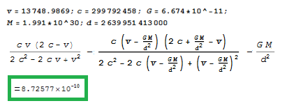
Which is almost exactly what JPL found at the epoch.

V – Decreasing difference

Now if we change for the velocity and distance of almost two months later so for example February the 21th of 1979 with v= 13729.7344 m.s^-1 and d = 2 701 676 943 000 we now found an anomaly of only 8.32453.10^-10 m/s²

And more than two year and a half later on October the 10th of 1981, v = 13 360.8107 m.s^-1, d = 3 827 209 369 000 and we find less than half of what we add at the beginning: 4.08073.10^-10 m/s²

The difference between the speed variation and the gravitation is exponentially decreasing:

But they naturally thought that this offset of unknown origin should be constant at around 8.7.10^-10 m.sec^-2. In the total absence of explanation on the origin of a phenomenon that was found precisely on a certain date we are inclined to think that it will be exactly the « same value » later as it’s the « same phenomenon ».

And from that moment they began to literally search this exactly offset of 8.7.10^-10 m.sec^-2 in all subsequent calculations. But the anomaly was less and less important in reality. This is a rather exemplary case of the experimenter effect, where a scientist makes his experimental results tend towards the result he seeks.

VI – Earth movement

At this point, and in those new conditions, it’s important to remind that the up trip of the signal, from Earth to the probe, is potentially influenced by the velocity of the Earth around the Sun from -30 km.s^-1 to +30 km.s^-1 depending on the period of the year.

Here is the well identified by JPL Doppler shift year variation due to the Earth movement:

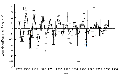
Even if the variation equilibrate itself in average from -30 km.s^-1 to +30 km.s^-1 I’m not sure to well understand why it has not been also considered as an anomaly at the epoch…

VII – Conclusion

Changing the relativistic formula (3) for the classic Galilean formula (5) in the Doppler shift calculation is equivalent to say that the electromagnetic wave obey to the velocities addition in a Galilean referential in some certain conditions (vacuum, no gravity, …).

Anderson wisely speculated that this would be interesting if the Pioneer anomaly was new physics, and perhaps after studying more deeply the hypothesis proposed in this article we’ll have to change the second postulate to something like:

Electromagnetic wave obey to the velocity addition and are emitted by the matter which produce them at the exact speed of c in their reference frame and in vacuum (without any Lorentz transformation of course).

We will have to study also if, has I think, in the case of a reflection, the new law apply on the emitted signal by the mirror, whatever the incoming signal velocity is.

L’anomalie de Pioneer 10 remet en cause le 2eme postulat d’Einstein

En se basant sur l’accélération anormale agissant sur Pioneer 10 avec une magnitude de 8,7×10-10 m/s² dirigée vers le Soleil, on peut démontrer qu’il existe une sérieuse indication que l’anomalie est due à l’utilisation d’une mauvaise formule de décalage Doppler par le Jet Propulsion Laboratory de la NASA (JPL).

En effet, si nous comparons le résultat donné par la formule relativiste basée sur le second postulat d’Einstein utilisée par JPL et le résultat donné par la formule classique d’addition de vitesse galiléenne, nous trouvons exactement la valeur de l’accélération anormale agissant sur Pioneer 10 vers le Soleil.

I – Comment avons-nous découvert la décélération anormale de 8.10−10 m/s² ?

Lors de la mission Pioneer 10, une station au sol envoyait un signal radio de fréquence ft, puis la sonde le renvoyait de manière synchrone à une station au sol qui le recevait à la fréquence fr.

Avec le décalage Doppler du signal radio, JPL (le Jet Propulsion Lab) était en mesure de calculer très précisément la vitesse de la sonde, et avec l’évolution de la vitesse ils pouvaient calculer l’accélération, qui était plus précisément une décélération puisque la sonde était attirée par l’ensemble du système solaire.

Avec cette attraction, selon la loi universelle de la gravitation et les positions bien connues du Soleil, des planètes et leurs masses, ils pouvaient calculer très précisément la distance qui nous séparait de la sonde.

Le problème est qu’une seconde plus tard, la vitesse de la sonde aurait dû décélérer exactement de l’attraction de gravité qu’ils venaient de calculer, mais non, elle avait décéléré un peu plus, d’environ 8,7.10−10 m / s², et même si c’est vraiment un tout petit peu plus, ce n’était pas normal.

II – Formule de décalage Doppler relativiste utilisée par JPL

La formule utilisée par JPL était la formule de décalage Doppler relativiste bien connue qui est:

Avec fs la fréquence envoyée, fr la fréquence reçue, β=v / c et v la vitesse entre l’émetteur et le récepteur.

Comme il y a deux trajet pour le signal, jusqu’à la sonde et le retour à la station sol, la formule aller-retour total est la suivante:

Et c’est ainsi que JPL en a déduit la vitesse v de la sonde:

III – Formule de décalage Doppler galiléen classique:

Pour le trajet du signal vers la sonde, avec v la vitesse de la sonde s’éloignant de la Terre, (considérons temporairement que la Terre est stationnaire avec le Soleil car nous verrons que son mouvement s’équilibre sur le long terme, évoluant de -30 km.s^-1 à +30 km.s^-1) la formule est la suivante:

Pour le retour du signal, dans le référentiel galiléen classique, la sonde est stationnaire et envoie le signal avec la vitesse de c dans son repère vers la Terre qui s’éloigne d’elle avec la vitesse v, donc la formule de retour est la même, et la formule totale aller-retour est:

Considérons que les formules galiléennes sont les bonnes. Dans ce cas, JPL calculerait toujours la vitesse de sonde avec (3), mais la fréquence reçue fr dépendrait d’une « vitesse réelle » différente de celle trouvée par JPL et nous pouvons exprimer la vitesse calculée par JPL, Vjpl en fonction de la « vitesse réelle » v de la sonde (deux vitesses différentes, une « réelle » et une autre, qui serait fausse donc, « calculée par JPL ») :

Ce qui peut être simplifié sans dépendre de la fréquence initiale ft émise par:  :

IV – Calcul de l’attraction du système solaire:

Le système solaire attire la sonde selon la loi de gravitation universelle avec toutes ses masses M et la distance d de la sonde:

Comme (8) est l’accélération réelle, chaque seconde, la vitesse réelle est modifiée en v – a et la vitesse calculée par JPL Vjpl exprimée en fonction de la vitesse réelle change pour:

Dans un premier temps JPL observait simplement la décélération avec Vjpl – Vjpl2 qui est égal à (7) – (9) et en déduisait la distance entre Pioneer 10 et le barycentre solaire avec la gravité. Ensuite, chaque seconde suivante les deux valeurs, le changement de vitesse et la gravité auraient dû commencer à correspondre toutes les secondes.

Mais l’attraction trouvée avec la variation de vitesse chaque seconde était toujours supérieure à l’attraction de gravité… Et l’une des premières fois qu’ils étudièrent précisément cette accélération anormale, début 1979, lorsque la distance de la sonde était de 2 639 951 413 000 m et de sa vitesse 13 748,9869 m.s^-1 (source NASA Horizon) ils ont trouvé dans la variation de la vitesse une décélération de 8,74.10-10 m/s² supérieure par rapport à la gravité à cette distance.

Et si JPL a commis une erreur en utilisant la formule relativiste (3) au lieu de la formule classique galiléenne (5), l’erreur est exactement égale à:

(7) – (9) – (8)

En faisant le calcul (merci à Wolfram!) Nous trouvons:

Ce qui est exactement ce que JPL a trouvé à l’époque…

V – Différence décroissante

Maintenant, si nous changeons pour la vitesse et la distance de presque deux mois plus tard, par exemple le 21 février 1979 avec v = 13729.7344 m.s^-1 et d = 2 701 676 943 000, nous trouvons maintenant une anomalie de seulement 8.32453.10-10 m/s²

Et plus de deux ans et demi plus tard le 10 octobre 1981, v = 13 360,8107 m.s^-1, d = 3 827 209 369 000 et nous trouvons moins de la moitié de ce que nous avions au début: 4.08073.10 -10 m/s²

La différence entre la variation de vitesse et la gravitation diminue de façon exponentielle:

Mais ils ont naturellement pensé que ce décalage d’origine inconnue devait être constant autour de 8.7.10-10 m/s². Et cela se comprend, en l’absence totale d’explication sur l’origine d’un phénomène constaté précisément à une certaine date, nous sommes enclins à penser que ce sera exactement la même valeur plus tard, puisqu’il s’agit à priori du « même phénomène ».

C’est ainsi qu’à partir de ce moment, ils ont commencé à chercher littéralement ce décalage exact de 8.7.10-10 m/s² dans tous les calculs ultérieurs. Mais l’anomalie était de moins en moins importante en réalité. C’est un cas assez exemplaire de l’effet expérimentateur, dans lequel un scientifique fait tendre ses résultats expérimentaux vers le résultat qu’il cherche.

VI – Mouvement de la Terre

Maintenant il est important de rappeler que le voyage aller du signal, de la Terre à la sonde, est potentiellement influencée par la vitesse de la Terre autour du Soleil de -30 km.s^-1 à + 30 km.s^-1 en fonction de la période de l’année. Et voici la variation annuelle bien identifiée du décalage Doppler due au mouvement de la Terre:

Même si la variation s’équilibre en moyenne de -30 km.s^-1 à +30 km.s^-1, je ne suis pas sûr de bien comprendre pourquoi elle n’a pas été considérée comme une anomalie à l’époque…

VII – Conclusion

Changer la formule relativiste (3) de la formule galiléenne classique (5) dans le calcul du décalage Doppler revient à dire que l’onde électromagnétique obéit à l’addition des vitesses dans un référentiel galiléen dans certaines conditions (vide, pas de gravité, …).

Anderson a judicieusement émis l’hypothèse que ce serait intéressant si l’anomalie de Pioneer était une nouvelle physique, et peut-être qu’après avoir étudié plus en profondeur l’hypothèse proposée ici, nous devrons changer le deuxième postulat en quelque chose comme:

Les ondes électromagnétiques obéissent à l’addition des vitesses et sont émises par la matière qui les produit à la vitesse exacte de c dans leur repère et dans le vide (sans transformation de Lorentz bien sûr).

Nous devrons également examiner si, comme je le pense, dans le cas d’une réflexion, la nouvelle loi s’applique au signal émis par le miroir, quelle que soit la vitesse du signal entrant.

SQL Process Explorer

Pour moi, sous Windows, l’application la plus importante à toujours été (de loin) Process Explorer de Mark Russinovich, alors quand j’ai commencer a remplir des fonctions de DBA un programme similaire m’a immédiatement manqué pour superviser SQL Server.

Comme j’ai été un développeur (depuis le ZX81 il y a quelques années ;) ) avant de devenir DBA j’ai fini par décider de faire un moi même une application de monitoring pour SQL Server. Et puisque j’ai toujours été reconnaissant à Mark pour la gratuité (et la qualité) de son travail, c’est maintenant mon tour d’offrir mon programme à ceux qui le voudront :

Le programme ne nécessite pas d’installation (comme procexp), c’est un simple executable .NET Framework 3.5 Client profile x86 (~400 Ko) :

Historique des versions

Il peut donc être lancer de n’importe quel répertoire (dans lequel il va générer un fichier .config pour enregistrer vos paramètres).

Le mode de capture principal est basé sur sys.sysprocesses, sys.dm_exec_requests et sys.dm_exec_sessions et double cliquer sur une ligne de la liste bascule sur l’onglet « Query » pour visualiser la requête et la ré-exécuter si besoin :

Les plus hauts niveaux de CPU, logical read, physical read, write, Wait time, Signal wait et 2 liste de wait configurable sont historisés. En passant la souris sur les histograms on obtient les informations de cette période avec la requête SQL qui était exécuté à ce moment par le process le plus consommateur du compteur concerné :

Il est donc simple de voir ce qu’il se passe en temps réel sur une instance, ou à un n’importe quel moment passé enregistré.

Les 2 listes de waits configurables sont par défaut (le titre se trouve avant les ‘:’ et les waits surveillés sont séparés avec des ‘;’ ensuite) :

IOWait:WRITELOG;IO_COMPLETION;PAGEIOLATCH_DT;PAGEIOLATCH_EX;PAGEIOLATCH_KP;PAGEIOLATCH_SH;PAGEIOLATCH_UP;ASYNC_IO_COMPLETION;

CXPacket:CXPACKET

J’ai ajouté un mode de capture expérimental basé sur la vue sys.dm_exec_query_stats (group by query_hash). Ce mode est accessible dans le menu option :

Dans ce mode, vous pouvez voir en violet les requêtes exécutées en parallèle, avec un elapsed time inférieur au worker time (pas une méthode parfaite je dois admettre).

Voilà, après cette petite introduction il ne vous reste plus qu’a l’expérimenter par vous même, en espérant que ça vous sera aussi utile qu’a moi. Si vous avez des idées je suis ouvert à toutes les propositions d’amélioration et si vous trouvez des bugs vous pouvez les signaler dans les commentaires de cette page ou par mail : sqlprocexp@gmail.com

 

SQL Process Explorer

For me, under Windows, the most important application has always been (by far) Process Explorer by Mark Russinovich, so when I started to assume DBA functions a similar program immediately missed me to monitor SQL Server.

As I was a developer (starting with the ZX81 a few years ago ;) ) before becoming DBA, I finally decided to make one myself. And since I’ve always been so thankful to Mark for his work (of such a quality) to be free, it is now my turn to offer freely my monitoring application for SQL Server to anyone who wants :

It doesn’t need any installation (as procexp), it’s a simple standalone .NET executable file Framework 3.5 Client profile x86 (~400 Ko) :

Version history

So it can be launch from any directory (in witch it will generate a .config file to save your parameters).

The main capture mode is based on sys.sysprocesses, sys.dm_exec_requests, and sys.dm_exec_sessions. Double-clicking on a row in the list show the « Query » tab to review the query and re-run if necessary:

The highest level of CPU, logical read, physical read, write, Wait Time, Signal wait, and 2 users configurables list of waits are historized and by passing the mouse over the histograms we obtain the information of this period with the SQL query that was executed at that time by the most consuming process of the counter concerned:

It’s then simple to see what is currently happening on the instance, or at any time recorded in the past.

The default user configurable waits are (before ‘:’ is the title of the wait and after separate with ‘;’ are the monitored waits) :

IOWait:WRITELOG;IO_COMPLETION;PAGEIOLATCH_DT;PAGEIOLATCH_EX;PAGEIOLATCH_KP;PAGEIOLATCH_SH;PAGEIOLATCH_UP;ASYNC_IO_COMPLETION;

CXPacket:CXPACKET

I’ve added an experimental capture mode based on the sys.dm_exec_query_stats view (group by query_hash). This mode is accessible in the option menu:

In this mode you can see in purple the query executed in parallel, with elapsed time lower than worker time (not a perfect method I must admit).

Here we are, after this quick introduction you should now experiment it by yourself, hoping that it will be as useful to you as it is to me. If you have ideas I am open to all suggestions for improvement and if you find bugs you can post them in the comments of this page or by mail : sqlprocexp@gmail.com